Tag: errors

  • Error Propagation and Conditioning

    Error Propagation and Conditioning

    In numerical computations, errors can propagate through calculations, potentially leading to significant inaccuracies in results. Understanding how errors propagate and how the conditioning of a problem affects numerical stability is crucial for designing robust numerical algorithms. In this post, I will discuss error propagation and the concept of conditioning in numerical problems.

    Error Propagation

    Errors in numerical computations arise from round-off errors, truncation errors, and uncertainties in input data. These errors can propagate through subsequent calculations, amplifying or dampening their effects depending on the nature of the problem and the algorithm used.

    Types of Error Propagation

    • Additive Propagation: When independent errors accumulate linearly through computations. For example, in summing a sequence of numbers, each with a small error, the total error grows proportionally.
    • Multiplicative Propagation: When errors are scaled through multiplication, leading to potentially exponential growth in error magnitude.
    • Differential Propagation: When small input errors lead to large output variations, particularly in functions with steep gradients.

    Example of Error Propagation

    Consider computing a function using finite differences: \(f'(x) \approx \frac{f(x+h) – f(x)}{h}\)

    If \(f(x)\) is obtained from measurements with small uncertainty, then errors in \(f(x+h)\) and \(f(x)\) propagate through the division by \(h\), potentially amplifying inaccuracies when \(h\) is very small.

    Conditioning of a Problem

    The conditioning of a numerical problem refers to how sensitive its solution is to small changes in the input. A well-conditioned problem has solutions that change only slightly with small perturbations in the input, whereas an ill-conditioned problem exhibits large variations in output due to small input changes.

    Measuring Conditioning: The Condition Number

    For a function \(f(x)\), the condition number \(\kappa\) measures how small relative errors in the input propagate to relative errors in the output: \(\kappa = \left| \frac{x}{f(x)} \frac{df(x)}{dx} \right|\)

    For matrix problems, the condition number is defined in terms of the matrix norm: \(\kappa(A) = \| A \| \cdot \| A^{-1} \|\)

    A high condition number indicates an ill-conditioned problem where small errors in input can lead to large deviations in the solution.

    Example of an Ill-Conditioned Problem

    Solving a nearly singular system of linear equations: \(Ax = b\)

    If the matrix \(A\) has a very large condition number, small perturbations in \(b\) or rounding errors can lead to vastly different solutions \(x\), making numerical methods unreliable.

    Visualizing Conditioning with a Function

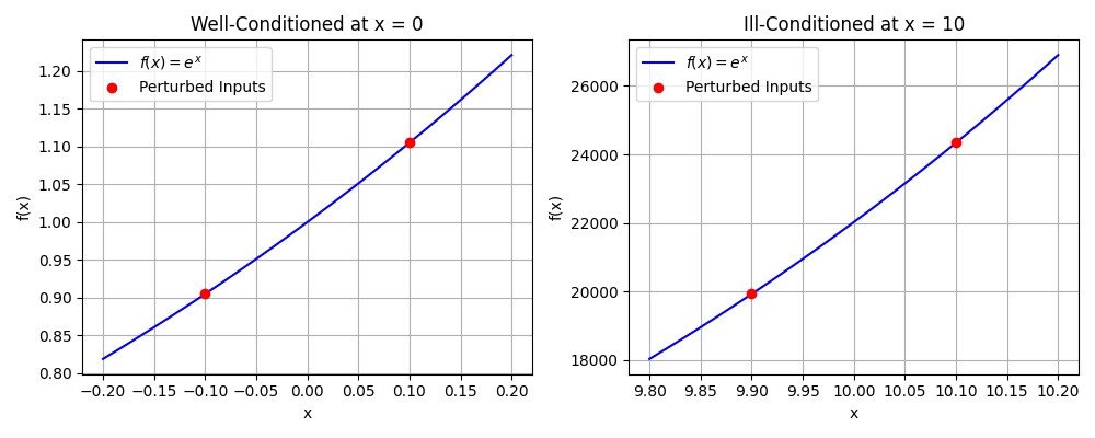
    To illustrate the concept of conditioning, consider the function \(f(x) = e^x\). The sensitivity of this function to input changes depends on the value of \(x\):

    • Well-Conditioned at \(x = 0\): Small changes in \(x\) (e.g., \(x = -0.1\) to \(x = 0.1\)) lead to small changes in \(f(x)\), indicating a well-conditioned problem.
    • Ill-Conditioned at \(x = 10\): Small changes in \(x\) (e.g., \(x = 9.9\) to \(x=10.1\)) cause large changes in \(f(x)\), illustrating an ill-conditioned problem.

    The following figure visually demonstrates this concept, where small perturbations in the input lead to significantly different outputs in ill-conditioned cases while remaining controlled in well-conditioned ones.
    Stability and Conditioning

    While conditioning is an inherent property of a problem, stability refers to how well an algorithm handles errors. A stable algorithm minimizes error amplification even when solving an ill-conditioned problem.

    Example of Algorithm Stability

    For solving linear systems \(Ax = b\), Gaussian elimination with partial pivoting is more stable than straightforward Gaussian elimination, as it reduces the impact of round-off errors on ill-conditioned systems.

    Conclusion

    Understanding error propagation and problem conditioning is essential for reliable numerical computations. While some problems are inherently sensitive to input errors, choosing numerically stable algorithms helps mitigate these effects. In the next post, I will discuss techniques for controlling numerical errors and improving computational accuracy.

  • Sources of Numerical Errors (Round-Off, Truncation, Stability)

    Sources of Numerical Errors (Round-Off, Truncation, Stability)

    Numerical computations inherently involve errors due to the limitations of representing and manipulating numbers in a finite-precision system. Understanding the different types of numerical errors is crucial for developing stable and accurate numerical algorithms. In this post, I will discuss three primary sources of numerical errors: round-off errors, truncation errors, and numerical stability.

    Round-Off Errors

    Round-off errors arise from the finite precision used to store numbers in a computer. Since most real numbers cannot be represented exactly in floating-point format, they must be approximated, leading to small discrepancies.

    Causes of Round-Off Errors

    • Finite Precision Representation: Floating-point numbers are stored using a limited number of bits, which results in small approximations for many numbers. For example, the decimal 0.1 cannot be exactly represented in binary, leading to a small error.
    • Arithmetic Operations: When performing arithmetic on floating-point numbers, small errors can accumulate.
    • Conversion Between Number Bases: Converting between decimal and binary introduces small inaccuracies due to repeating fractions in binary representation.

    Example of Round-Off Error

    Consider summing 0.1 ten times in floating-point arithmetic:

    import numpy as np
    print(sum([0.1] * 10) == 1.0)  # Expected True, but may return False due to precision error
    print(sum([0.1] * 10))  # Output: 0.9999999999999999

    This error occurs because 0.1 is stored as an approximation, and the accumulation of small errors results in a slight deviation from 1.0.

    Catastrophic Cancellation

    Catastrophic cancellation is a specific type of round-off error that occurs when subtracting two nearly equal numbers. Since the leading significant digits cancel out, the result has significantly reduced precision, often leading to large relative errors.

    For example, consider:

    import numpy as np
    x = np.float32(1.0000001)
    y = np.float32(1.0000000)
    print(x - y)  # Loss of significant digits due to cancellation

    If the subtraction results in a number much smaller than the original values, relative errors become large, reducing numerical accuracy. This type of error is especially problematic in iterative methods and when computing small differences in large values.

    Truncation Errors

    Truncation errors occur when an infinite or continuous mathematical process is approximated by a finite or discrete numerical method. These errors arise from simplifying mathematical expressions or using approximate numerical techniques.

    Causes of Truncation Errors

    • Numerical Differentiation and Integration: Approximating derivatives using finite differences or integrals using numerical quadrature leads to truncation errors.
    • Series Expansions: Many functions are approximated using truncated Taylor series expansions, leading to errors that depend on the number of terms used.
    • Discretization of Continuous Problems: Solving differential equations numerically involves discretizing time or space, introducing truncation errors.

    Example of Truncation Error

    Approximating the derivative of \(f(x) = \sin(x)\) using the finite difference formula: \(f'(x) \approx \frac{f(x+h) – f(x)}{h}\)

    For small h, this formula provides an approximation, but it is not exact because it ignores higher-order terms in the Taylor series expansion.

    Numerical Stability

    Numerical stability pertains to an algorithm’s sensitivity to small perturbations, such as round-off or truncation errors, during its execution. A numerically stable algorithm ensures that such small errors do not grow uncontrollably, thereby maintaining the accuracy of the computed results.

    Causes of Numerical Instability

    • Ill-Conditioned Problems: Some problems are highly sensitive to small changes in input. For example, solving a nearly singular system of linear equations can magnify errors, making the solution highly inaccurate.
    • Unstable Algorithms: Some numerical methods inherently amplify errors during execution. For instance, certain iterative solvers may diverge rather than converge if they are not properly designed.
    • Accumulation of Round-Off Errors in Repeated Computations: When an algorithm involves repeated arithmetic operations, small round-off errors may compound over time, leading to significant deviations from the true result.

    Example of Numerical Instability: Iterative Methods

    Consider an iterative method designed to approximate the square root of a number. If the method is not properly formulated, small errors in each iteration can accumulate, leading to divergence from the true value rather than convergence. This behavior exemplifies numerical instability, as the algorithm fails to control the propagation of errors through successive iterations.

    Conclusion

    Understanding numerical errors is crucial for designing reliable computational methods. While round-off errors stem from finite precision representation, truncation errors arise from approximations in numerical methods. Stability plays a key role in determining whether small errors will remain controlled or grow exponentially. In the next post, I will discuss techniques to mitigate these errors and improve numerical accuracy.