Theoretical Insights

Category: numerical techniques

Error Propagation and Conditioning
In numerical computations, errors can propagate through calculations, potentially leading to significant inaccuracies in results. Understanding how errors propagate and how the conditioning of a problem affects numerical stability is crucial for designing robust numerical algorithms. In this post, I will discuss error propagation and the concept of conditioning in numerical problems.

Error Propagation

Errors in numerical computations arise from round-off errors, truncation errors, and uncertainties in input data. These errors can propagate through subsequent calculations, amplifying or dampening their effects depending on the nature of the problem and the algorithm used.

Types of Error Propagation
- Additive Propagation: When independent errors accumulate linearly through computations. For example, in summing a sequence of numbers, each with a small error, the total error grows proportionally.
- Multiplicative Propagation: When errors are scaled through multiplication, leading to potentially exponential growth in error magnitude.
- Differential Propagation: When small input errors lead to large output variations, particularly in functions with steep gradients.
Example of Error Propagation

Consider computing a function using finite differences: \(f'(x) \approx \frac{f(x+h) – f(x)}{h}\)

If \(f(x)\) is obtained from measurements with small uncertainty, then errors in \(f(x+h)\) and \(f(x)\) propagate through the division by \(h\), potentially amplifying inaccuracies when \(h\) is very small.

Conditioning of a Problem

The conditioning of a numerical problem refers to how sensitive its solution is to small changes in the input. A well-conditioned problem has solutions that change only slightly with small perturbations in the input, whereas an ill-conditioned problem exhibits large variations in output due to small input changes.

Measuring Conditioning: The Condition Number

For a function \(f(x)\), the condition number \(\kappa\) measures how small relative errors in the input propagate to relative errors in the output: \(\kappa = \left| \frac{x}{f(x)} \frac{df(x)}{dx} \right|\)

For matrix problems, the condition number is defined in terms of the matrix norm: \(\kappa(A) = \| A \| \cdot \| A^{-1} \|\)

A high condition number indicates an ill-conditioned problem where small errors in input can lead to large deviations in the solution.

Example of an Ill-Conditioned Problem

Solving a nearly singular system of linear equations: \(Ax = b\)

If the matrix \(A\) has a very large condition number, small perturbations in \(b\) or rounding errors can lead to vastly different solutions \(x\), making numerical methods unreliable.

Visualizing Conditioning with a Function

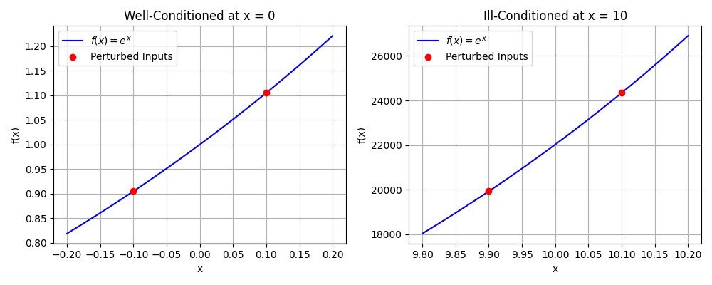
To illustrate the concept of conditioning, consider the function \(f(x) = e^x\). The sensitivity of this function to input changes depends on the value of \(x\):
- Well-Conditioned at \(x = 0\): Small changes in \(x\) (e.g., \(x = -0.1\) to \(x = 0.1\)) lead to small changes in \(f(x)\), indicating a well-conditioned problem.
- Ill-Conditioned at \(x = 10\): Small changes in \(x\) (e.g., \(x = 9.9\) to \(x=10.1\)) cause large changes in \(f(x)\), illustrating an ill-conditioned problem.
The following figure visually demonstrates this concept, where small perturbations in the input lead to significantly different outputs in ill-conditioned cases while remaining controlled in well-conditioned ones.

Stability and Conditioning

While conditioning is an inherent property of a problem, stability refers to how well an algorithm handles errors. A stable algorithm minimizes error amplification even when solving an ill-conditioned problem.

Example of Algorithm Stability

For solving linear systems \(Ax = b\), Gaussian elimination with partial pivoting is more stable than straightforward Gaussian elimination, as it reduces the impact of round-off errors on ill-conditioned systems.

Conclusion

Understanding error propagation and problem conditioning is essential for reliable numerical computations. While some problems are inherently sensitive to input errors, choosing numerically stable algorithms helps mitigate these effects. In the next post, I will discuss techniques for controlling numerical errors and improving computational accuracy.
10 July 2025
Sources of Numerical Errors (Round-Off, Truncation, Stability)
Numerical computations inherently involve errors due to the limitations of representing and manipulating numbers in a finite-precision system. Understanding the different types of numerical errors is crucial for developing stable and accurate numerical algorithms. In this post, I will discuss three primary sources of numerical errors: round-off errors, truncation errors, and numerical stability.

Round-Off Errors

Round-off errors arise from the finite precision used to store numbers in a computer. Since most real numbers cannot be represented exactly in floating-point format, they must be approximated, leading to small discrepancies.

Causes of Round-Off Errors
- Finite Precision Representation: Floating-point numbers are stored using a limited number of bits, which results in small approximations for many numbers. For example, the decimal 0.1 cannot be exactly represented in binary, leading to a small error.
- Arithmetic Operations: When performing arithmetic on floating-point numbers, small errors can accumulate.
- Conversion Between Number Bases: Converting between decimal and binary introduces small inaccuracies due to repeating fractions in binary representation.
Example of Round-Off Error

Consider summing 0.1 ten times in floating-point arithmetic:
```
import numpy as np
print(sum([0.1] * 10) == 1.0)  # Expected True, but may return False due to precision error
print(sum([0.1] * 10))  # Output: 0.9999999999999999
```
This error occurs because 0.1 is stored as an approximation, and the accumulation of small errors results in a slight deviation from 1.0.

Catastrophic Cancellation

Catastrophic cancellation is a specific type of round-off error that occurs when subtracting two nearly equal numbers. Since the leading significant digits cancel out, the result has significantly reduced precision, often leading to large relative errors.

For example, consider:
```
import numpy as np
x = np.float32(1.0000001)
y = np.float32(1.0000000)
print(x - y)  # Loss of significant digits due to cancellation
```
If the subtraction results in a number much smaller than the original values, relative errors become large, reducing numerical accuracy. This type of error is especially problematic in iterative methods and when computing small differences in large values.

Truncation Errors

Truncation errors occur when an infinite or continuous mathematical process is approximated by a finite or discrete numerical method. These errors arise from simplifying mathematical expressions or using approximate numerical techniques.

Causes of Truncation Errors
- Numerical Differentiation and Integration: Approximating derivatives using finite differences or integrals using numerical quadrature leads to truncation errors.
- Series Expansions: Many functions are approximated using truncated Taylor series expansions, leading to errors that depend on the number of terms used.
- Discretization of Continuous Problems: Solving differential equations numerically involves discretizing time or space, introducing truncation errors.
Example of Truncation Error

Approximating the derivative of \(f(x) = \sin(x)\) using the finite difference formula: \(f'(x) \approx \frac{f(x+h) – f(x)}{h}\)

For small h, this formula provides an approximation, but it is not exact because it ignores higher-order terms in the Taylor series expansion.

Numerical Stability

Numerical stability pertains to an algorithm’s sensitivity to small perturbations, such as round-off or truncation errors, during its execution. A numerically stable algorithm ensures that such small errors do not grow uncontrollably, thereby maintaining the accuracy of the computed results.

Causes of Numerical Instability
- Ill-Conditioned Problems: Some problems are highly sensitive to small changes in input. For example, solving a nearly singular system of linear equations can magnify errors, making the solution highly inaccurate.
- Unstable Algorithms: Some numerical methods inherently amplify errors during execution. For instance, certain iterative solvers may diverge rather than converge if they are not properly designed.
- Accumulation of Round-Off Errors in Repeated Computations: When an algorithm involves repeated arithmetic operations, small round-off errors may compound over time, leading to significant deviations from the true result.
Example of Numerical Instability: Iterative Methods

Consider an iterative method designed to approximate the square root of a number. If the method is not properly formulated, small errors in each iteration can accumulate, leading to divergence from the true value rather than convergence. This behavior exemplifies numerical instability, as the algorithm fails to control the propagation of errors through successive iterations.

Conclusion

Understanding numerical errors is crucial for designing reliable computational methods. While round-off errors stem from finite precision representation, truncation errors arise from approximations in numerical methods. Stability plays a key role in determining whether small errors will remain controlled or grow exponentially. In the next post, I will discuss techniques to mitigate these errors and improve numerical accuracy.
20 March 2025
Representation of Numbers in Computers
Computers handle numbers differently from how we do in mathematics. While we are accustomed to exact numerical values, computers must represent numbers using a finite amount of memory. This limitation leads to approximations, which can introduce errors in numerical computations. In this post, I will explain how numbers are stored in computers, focusing on integer and floating-point representations.

Integer Representation

Integers are stored exactly in computers using binary representation. Each integer is stored in a fixed number of bits, commonly 8, 16, 32, or 64 bits. The two primary representations of integers are:

The Binary System

Computers operate using binary (base-2) numbers, meaning they represent all values using only two digits: 0 and 1. Each digit in a binary number is called a bit. The value of a binary number is computed similarly to decimal (base-10) numbers but using powers of 2 instead of powers of 10.

For example, the binary number 1101 represents: \[(1 \times 2^3)+(1 \times 2^2)+(0 \times 2^1)+(1 \times 2^0)=8+4+0+1=13\]

Similarly, the decimal number 9 is represented in binary as 1001.

Unsigned Integers

Unsigned integers can only represent non-negative values. A n-bit unsigned integer can store values from 0 to 2^n - 1. For example, an 8-bit unsigned integer can represent values from 0 to 255 (2^8 - 1).

Signed Integers and Two’s Complement

Signed integers can represent both positive and negative numbers. The most common way to store signed integers is two’s complement, which simplifies arithmetic operations and ensures unique representations for zero.

In two’s complement representation:
- The most significant bit (MSB) acts as the sign bit (0 for positive, 1 for negative).
- Negative numbers are stored by taking the binary representation of their absolute value, inverting the bits, and adding 1.
For example, in an 8-bit system:
- +5 is represented as 00000101
- -5 is obtained by:
  1. Writing 5 in binary: 00000101
  2. Inverting the bits: 11111010
  3. Adding 1: 11111011
Thus, -5 is stored as 11111011.

One of the key advantages of two’s complement is that subtraction can be performed as addition. For instance, computing 5 - 5 is the same as 5 + (-5), leading to automatic cancellation without requiring separate subtraction logic in hardware.

The range of a n-bit signed integer is from -2^(n-1) to 2^(n-1) - 1. For example, an 8-bit signed integer ranges from -128 to 127.

Floating-Point Representation

Most real numbers cannot be represented exactly in a computer due to limited memory. Instead, they are stored using the IEEE 754 floating-point standard, which represents numbers in the form: \[x = (-1)^s \times M \times 2^E\]

where:
- s is the sign bit (0 for positive, 1 for negative).
- M (the mantissa) stores the significant digits.
- E (the exponent) determines the scale of the number.
How the Mantissa and Exponent Are Stored and Interpreted

The mantissa (also called the significand) and exponent are stored in a structured manner to ensure a balance between precision and range.
- Mantissa (Significand): The mantissa represents the significant digits of the number. In IEEE 754, the mantissa is stored in normalized form, meaning that the leading bit is always assumed to be 1 (implicit bit) and does not need to be stored explicitly. This effectively provides an extra bit of precision.
- Exponent: The exponent determines the scaling factor for the mantissa. It is stored using a bias system to accommodate both positive and negative exponents.
  - In single precision (32-bit): The exponent uses 8 bits with a bias of 127. This means the stored exponent value is E + 127.
  - In double precision (64-bit): The exponent uses 11 bits with a bias of 1023. The stored exponent value is E + 1023.
For example, the decimal number 5.75 is stored in IEEE 754 single precision as:
1. Convert to binary: 5.75 = 101.11_2
2. Normalize to scientific notation: 1.0111 × 2^2
3. Encode:
  - Sign bit: 0 (positive)
  - Exponent: 2 + 127 = 129 (binary: 10000001)
  - Mantissa: 01110000000000000000000 (without the leading 1)
Final representation in binary: 0 10000001 01110000000000000000000

Special Floating-Point Values: Inf and NaN

IEEE 754 also defines special representations for infinite values and undefined results:
- Infinity (Inf): This occurs when a number exceeds the largest representable value. It is represented by setting the exponent to all 1s and the mantissa to all 0s:
  - Positive infinity: 0 11111111 00000000000000000000000
  - Negative infinity: 1 11111111 00000000000000000000000
- Not-a-Number (NaN): This is used to represent undefined results such as 0/0 or sqrt(-1). It is identified by an exponent of all 1s and a nonzero mantissa:
  - NaN: x 11111111 ddddddddddddddddddddddd (where x is the sign bit and d is any nonzero value in the mantissa)
Subnormal Numbers

Subnormal numbers (also called denormalized numbers) are a special category of floating-point numbers used to represent values that are too small to be stored in the normal format. They help address the issue of underflow, where very small numbers would otherwise be rounded to zero.

Why Are Subnormal Numbers Needed?

In standard IEEE 754 floating-point representation, the smallest normal number occurs when the exponent is at its minimum allowed value. However, values smaller than this minimum would normally be rounded to zero, causing a loss of precision in numerical computations. To mitigate this, IEEE 754 defines subnormal numbers, which allow for a gradual reduction in precision rather than an abrupt transition to zero.

How Are Subnormal Numbers Represented?

A normal floating-point number follows the form: \[x = (-1)^s \times (1 + M) \times 2^E\]

where 1 + M represents the implicit leading bit (always 1 for normal numbers), and E is the exponent.

For subnormal numbers, the exponent is set to the smallest possible value (E = 1 - bias), and the leading 1 in the mantissa is no longer assumed. Instead, the number is stored as: \[x = (-1)^s \times M \times 2^{1 – \text{bias}}\]

This means subnormal numbers provide a smooth transition from the smallest normal number to zero, reducing sudden underflow errors.

Example of a Subnormal Number

In IEEE 754 single-precision (32-bit) format:
- The smallest normal number occurs when E = 1 (after subtracting bias: E - 127 = -126).
- The next smaller numbers are subnormal, where E = 0, and the mantissa gradually reduces towards zero.
For example, a subnormal number with a small mantissa could look like:
```
0 00000000 00000000000000000000001
```
This represents a very small positive number, much closer to zero than any normal number.

Limitations of Subnormal Numbers
- They have reduced precision, as the leading 1 bit is missing.
- Operations involving subnormal numbers are often slower on some hardware due to special handling.
- In extreme cases, they may still lead to precision loss in calculations.
Precision and Limitations

Floating-point representation allows for a vast range of values, but it comes with limitations:
- Finite Precision: Only a finite number of real numbers can be represented.
- Rounding Errors: Some numbers (e.g., 0.1 in binary) cannot be stored exactly, leading to small inaccuracies.
- Underflow and Overflow: Extremely small numbers may be rounded to zero (underflow), while extremely large numbers may exceed the maximum representable value (overflow).
Example: Floating-Point Approximation

Consider storing 0.1 in a 32-bit floating-point system. Its binary representation is repeating, meaning it must be truncated, leading to a slight approximation error. This small error can propagate in calculations, affecting numerical results.

Conclusion

Understanding how numbers are represented in computers is crucial in computational physics and numerical methods. In the next post, I will explore sources of numerical errors, including truncation and round-off errors, and how they impact computations.
13 March 2025
Overview of Python and C++ for Scientific Computing
When it comes to scientific computing, Python and C++ are two of the most widely used programming languages. Each has its own strengths and weaknesses, making them suitable for different types of computational tasks. In this post, I will compare these languages, discuss essential libraries, and outline a basic workflow for implementing numerical methods in both.

Strengths and Weaknesses of Python and C++ in Computational Physics

Python

Strengths:
- Easy to learn and use, making it ideal for rapid prototyping
- Rich ecosystem of scientific libraries (NumPy, SciPy, SymPy, Matplotlib, etc.)
- High-level syntax that makes code more readable and concise
- Strong community support and extensive documentation
- Good for data analysis, visualization, and scripting
Weaknesses:
- Slower execution speed due to being an interpreted language
- Not well-suited for real-time or highly parallelized computations without additional frameworks (e.g., Cython, Numba, or TensorFlow)
- Limited control over memory management compared to C++
C++

Strengths:
- High-performance execution, making it suitable for computationally intensive simulations
- Fine-grained control over memory management and hardware resources
- Strongly typed language, reducing runtime errors
- Optimized numerical libraries such as Eigen and Boost
- Suitable for large-scale scientific computing and high-performance computing (HPC) applications
Weaknesses:
- Steeper learning curve compared to Python
- More complex syntax, making code harder to write and maintain
- Slower development time due to manual memory management and debugging
- Requires explicit compilation before execution
Key Libraries and Tools

Both Python and C++ have extensive libraries that facilitate numerical computations in physics:

Python Libraries:
- NumPy: Provides fast array operations and linear algebra routines
- SciPy: Extends NumPy with additional numerical methods (optimization, integration, ODE solvers, etc.)
- SymPy: Symbolic computation library for algebraic manipulations
- Matplotlib: Essential for data visualization and plotting results
C++ Libraries:
- Eigen: High-performance linear algebra library
- Boost: Collection of advanced numerical and utility libraries
- Armadillo: A convenient linear algebra library with a syntax similar to MATLAB
- FFTW: Optimized library for computing fast Fourier transforms
Basic Workflow of Implementing a Numerical Method in Python and C++

The workflow for implementing a numerical method follows a similar structure in both languages, though the execution and syntax differ.

Python Workflow:
1. Import necessary libraries (e.g., NumPy, SciPy)
2. Define the function to implement the numerical method
3. Apply the method to a physics problem
4. Visualize the results using Matplotlib
5. Optimize performance using tools like NumPy vectorization or Numba
Example (Numerical Integration using Python):
```
import numpy as np
from scipy.integrate import quad

def function(x):
    return np.sin(x)

result, error = quad(function, 0, np.pi)
print("Integral:", result)
```
C++ Workflow:
1. Include necessary libraries (e.g., Eigen, Boost)
2. Define functions and structures for numerical computation
3. Implement the numerical method using efficient algorithms
4. Compile the code with an appropriate compiler (e.g., g++)
5. Optimize performance using multi-threading, vectorization, or parallel processing
Example (Numerical Integration using C++ and Boost):
```
#include <iostream>
#include <boost/math/quadrature/trapezoidal.hpp>

double function(double x) {
    return sin(x);
}

int main() {
    double result = boost::math::quadrature::trapezoidal(function, 0.0, M_PI);
    std::cout << "Integral: " << result << std::endl;
    return 0;
}
```
Using Python for Development and C++ for Performance

When developing or testing new numerical schemes, it is often worthwhile to use Python initially before porting the final implementation to C++ for performance. This approach has several advantages:
- Faster Development Cycle: Python’s high-level syntax and extensive libraries allow for quick experimentation and debugging.
- Ease of Debugging: Python’s interpreted nature makes it easier to test and refine numerical methods without needing to recompile code.
- Rapid Prototyping: The ability to write concise, readable code means that algorithms can be validated efficiently before optimizing for performance.
- Hybrid Approach: Once an algorithm is validated, performance-critical parts can be rewritten in C++ for speed, either as standalone applications or as Python extensions using Cython or pybind11.
This hybrid workflow balances ease of development with execution efficiency, ensuring that numerical methods are both correct and optimized.

Brief Discussion on Performance Considerations

The choice between Python and C++ depends on the trade-off between development speed and execution performance.
- Python (Interpreted Language): Python is dynamically typed and interpreted, meaning it incurs runtime overhead but allows for quick experimentation and debugging.
- C++ (Compiled Language): C++ is statically typed and compiled, leading to significantly faster execution but requiring more effort in debugging and code optimization.
- Optimization Techniques: Python can be accelerated using JIT compilers like Numba, or by writing performance-critical components in C++ and calling them from Python using tools like Cython or pybind11.
Conclusion

Both Python and C++ are powerful tools for computational physics, each serving a different purpose. Python is excellent for prototyping, analysis, and visualization, while C++ is preferred for high-performance simulations and large-scale computations. In the next posts, I will demonstrate how to implement numerical methods in these languages, starting with basic root-finding algorithms.
6 March 2025
Bridging Theory and Computation: An Introduction to Computational Physics and Numerical Methods
Computational physics has become an indispensable tool in modern scientific research. As a physicist, I have encountered numerous problems where analytical solutions are either impractical or outright impossible. In such cases, numerical methods provide a powerful alternative, allowing us to approximate solutions to complex equations and simulate physical systems with remarkable accuracy.

What is Computational Physics?

At its core, computational physics is the application of numerical techniques to solve physical problems. It bridges the gap between theoretical physics and experimental physics, providing a way to test theories, explore new physical regimes, and analyze systems that are too complex for pen-and-paper calculations.

Unlike purely theoretical approaches, computational physics does not rely on closed-form solutions. Instead, it employs numerical algorithms to approximate the behavior of systems governed by differential equations, integral equations, or even stochastic processes. This approach has been instrumental in fields such as astrophysics, condensed matter physics, plasma physics, and quantum mechanics.

What are Numerical Methods?

Numerical methods are the mathematical techniques that underpin computational physics. These methods allow us to approximate solutions to problems that lack analytical expressions. Some of the most fundamental numerical techniques include:
- Root-finding algorithms (e.g., Newton-Raphson method)
- Solving systems of linear and nonlinear equations (e.g., Gaussian elimination, iterative solvers)
- Numerical differentiation and integration (e.g., finite difference methods, trapezoidal rule)
- Solving ordinary and partial differential equations (e.g., Euler’s method, Runge-Kutta methods, finite element methods)
- Monte Carlo methods for statistical simulations
Each of these methods comes with its own strengths and limitations, which must be carefully considered depending on the problem at hand. Computational physicists must be adept at choosing the appropriate numerical approach while ensuring stability, accuracy, and efficiency.

The Role of Computation in Modern Physics

Over the past few decades, computational physics has reshaped the way we approach scientific problems. Consider, for instance, the study of chaotic systems such as weather patterns or turbulence in fluids. These systems are governed by nonlinear equations that defy analytical treatment, but numerical simulations allow us to explore their dynamics in great detail. Similarly, in quantum mechanics, solving the Schrödinger equation for complex many-body systems would be infeasible without numerical approaches such as the density matrix renormalization group (DMRG) or quantum Monte Carlo methods.

Moreover, high-performance computing (HPC) has opened up new frontiers in physics. Supercomputers enable large-scale simulations of everything from galaxy formation to plasma confinement in nuclear fusion reactors. The interplay between numerical methods and computational power continues to drive progress in physics, allowing us to probe deeper into the fundamental nature of the universe.

Conclusion

Computational physics and numerical methods go hand in hand, forming a crucial pillar of modern scientific inquiry. In this course, I will introduce key numerical techniques, provide implementations in Python and C++, and apply them to real-world physics problems. By the end, you will not only understand the theoretical foundations of numerical methods but also gain hands-on experience in using them to tackle complex physical systems.

In the next post, I will delve deeper into the role of numerical computation in physics, exploring when and why numerical approaches are necessary and how they complement both theory and experiment.
27 February 2025